Meta-Learning with Julia & Flux

All the code can be found at this repo.

Transfer Learning is when the parameters of a neural network model previously trained on a task are used as as the starting parameters to train on a new task. The canonical use case being using a convolutional network trained on ImageNet to classify images and finetuning the final layer, or the entire model to classify new image categories, perform image segmentation, detect objects, etc. Very recently natural language has had its transfer learning epiphany with BERT, a pretrained model for language representations. A key difference between BERT and the ImageNet example is BERT is trained with the goal of "language understanding" whereas training a convolutional network on ImageNet stumbles upon a useful image representation since the goal is to classify images not "image understanding". Fundamentally, the goal of transfer learning is to learn a function which takes an input and outputs an useful embedding as an input for other functions.

Meta-Learning

Meta-Learning learns a function that learns functions.

A neural network to trained to perform image classification learns a function which receives an image as input and outputs a label. While this is a valuable function, it's heavily conditioned on images seen during training and typically fails to generalize to images of unseen classes. The meta-learning approach would be to train a neural network which is good at learning to classify images.

Could the original classification neural network learn to classify new images? Absolutely, but its not exactly that simple. How much data of the new class is required? How much longer must the network be trained? Will learning the new class hurt the overall classification performance?

The hope of meta-learning is to learn a new task with minimal additional data and training time. Revising the original description:

Meta-Learning learns a function that learns functions quickly with minimal data.

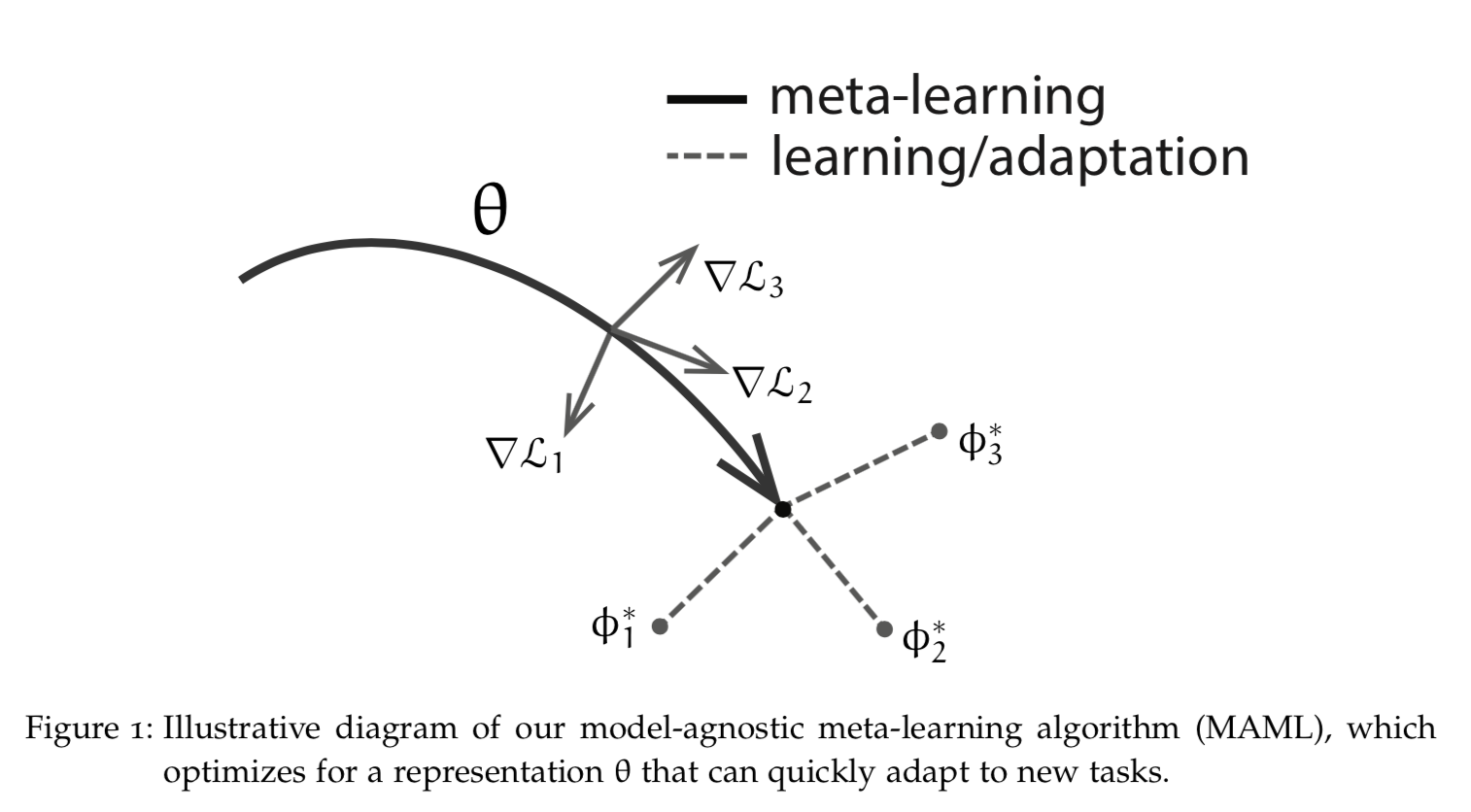
The above figure of MAML is from Chelsea B. Finn's Learning to Learn with Gradients. Reptile is the other algorithm we'll cover.

There are many possible representations a neural network can learn but there are few representations, $\theta^{*}$ which minimize the average distance and additional training time taken to a optimal solution for any task $t_{i}$ . This is representation we attempt to find with meta-learning.

MAML and Reptile consist of two objectives. The first minimizes the loss for a specific task and in doing so leends to teaching the parameters to learn quickly. The second uses information provided from the task specific objective to generalize to new tasks. Formal arguments for this can be found section 5 of the Reptile paper. This process is repeated until the neural network is good at learning to learn:

while true
    task = sample_task()
    info = optimize_for_task(task_loss, model_parameters, task)
    grads = optimize_for_meta_goal(meta_loss, model_parameters, task, info)
    model_parameters = update_parameters(model_parameters, grads)
end

Before we get into MAML and Reptile implementations let's go over the problem we're solving.

Problem Setup

We'll be using meta-learning to learn to learn sine waves!

This is a sine wave:

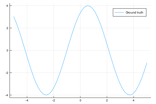
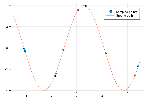
This is what we'd like the neural network to do, given a handful of points figure out the underlying sine wave the points originate from.

The sine waves will have the following form:

struct SineWave
    amplitude::Float32
    phase_shift::Float32
end
SineWave() = SineWave(rand(Uniform(0.1, 5)), rand(Uniform(0, 2pi)))

(s::SineWave)(x::AbstractArray) = s.amplitude .* sin.(x .+ s.phase_shift)

function Base.show(io::IO, s::SineWave)
    print(io, "SineWave(amplitude = ", s.amplitude, ", phase shift = ", s.phase_shift, ")")
end

where the amplitude shortens or lengthens the height of the wave and phase shift shifts the wave to the left or right.

If you're new to Julia don't fret, I'm a reasonably good Julia-Python translator :)

struct is analogous to Python's class.
SineWave() = SineWave(rand(Uniform(0.1, 5)), rand(Uniform(0, 2pi))) is a convenience constructor. Everytime SineWave() is called it will create a SineWave with an amplitude and phase shift sampled uniform distributions [0.1, 5] and [0, 2 $\pi$ ] respectively.
(s::SineWave)(x::AbstractArray) = s.amplitude .* sin.(x .+ s.phase_shift). (s::SineWave)(x::AbstractArray) roughly translates to this method of a SineWave class - def __call__(self, x): ... where x is a PyTorch Tensor
s.amplitude .* sin.(x .+ s.phase_shift). You may be wondering why there's a . before function calls. This signifies the function is applied elementwise.
Base.show is similar to def __repr(self, ...). It returns a string representation.

Example usage:

using Distributions

# sample 10 points from a uniform distribution [-5, 5]
julia> x = rand(Uniform(-5, 5), 10)
10-element Array{Float64,1}:
 -1.9279845796432626
 -2.565858434186461
 -0.8290583563692184
  0.32121125997540645
 -2.362361975212195
  2.9885150288281004
  4.728599209179194
  2.174174776306687
 -0.3368270599587264
  4.444254583770027

julia> wave = SineWave(4, 1)
SineWave(amplitude = 4.0, phase shift = 1.0)

julia> wave(x)
10-element Array{Float64,1}:
 -3.201653707457795
 -3.999951234532262
  0.6804413741673037
  3.8760599776431177
 -3.9134243632070027
 -2.9969826795933403
 -2.1063659183401633
 -0.1303054327518841
  2.462481437847728
 -2.9757159681499266

Unless otherwise stated the following model will be used:

using Flux
using MetaLearning

model = Chain(
   Linear(1, 64, tanh),
   Linear(64, 64, tanh),
   Linear(64, 1)
)

Linear is a slight modification of Dense. The modification is uses both the input and output dimension values to calculate bias initialization. All weights and biases are initialized with a uniform distribution initialization $[-\sigma, \sigma]$ with $\sigma$ defined as:

\sigma = \sqrt\frac{1}{n_{in}}

where $n_{in}$ is the input dimension. This is known as the Xavier initialization and it performed better than glorot_uniform initialization baked into Flux's Dense layer.

The above Flux architecture maps to the following in PyTorch:

import torch.nn as nn

model = nn.Sequential(
    nn.Linear(1, 64),
    nn.Tanh(),
    nn.Linear(64, 64),
    nn.Tanh(),
    nn.Linear(64, 1),
)

The following code evaluates the model on a sine wave task training to sample x with updates amount of gradient steps using opt. Unless otherwise stated finetuning involes 32 gradient update steps.

Evaluation loss is calculated based on the mean squared error between model predictions and sine wave values: Flux.mse(model(testx'), testy').

function eval_model(model, x::AbstractArray, testx::AbstractArray, task=SineWave();
                    opt=Descent(1e-2), updates=32)
    weights = params(model)
    prev_weights = deepcopy(Flux.data.(weights))

    y = task(x)
    testy = task(testx)
    init_preds = model(testx')
    test_loss = Flux.mse(init_preds, testy')

    test_losses = Float32[]
    push!(test_losses, Flux.data(test_loss))

    @printf(task)
    @printf("Before finetuning, Loss = %f\n", test_loss)
    for i in 1:updates
        l = Flux.mse(model(x'), y')
        Flux.back!(l)
        Flux.Optimise._update_params!(opt, weights)
        test_loss = Flux.mse(model(testx'), testy')
        push!(test_losses, Flux.data(test_loss))
        @printf("After %d fits, Loss = %f\n", i, test_loss)
    end
    final_preds = model(testx')

    Flux.loadparams!(model, prev_weights)

    return (x=x, testx=testx, y=y, testy=testy,
            initial_predictions=Array(Flux.data(init_preds)'),
            final_predictions=Array(Flux.data(final_preds)'),
            test_losses=test_losses)
end

The returned values are used for plotting with Plots:

using Plots

function plot_eval_data(data::NamedTuple, title="")
    return plot([data.x, data.testx, data.testx, data.testx],
                [data.y, data.testy, data.initial_predictions, data.final_predictions],
                line=[:scatter :path :path :path],
                label=["Sampled points", "Ground truth", "Before finetune", "After finetune"],
                foreground_color_legend=:white, background_color_legend=:transparent,
                title=title,
                xlim=(-5.5, 5.5))
end

Time for a Flux to PyTorch translation detour!

params(model) -> model.parameters()
Flux.mse -> torch.nn.functional.mse_loss
Flux.back!(l) -> l.backward()
Flux.Optimizer._update_params!(opt, weights) -> opt.step(); opt.zero_grad()

Experiments

Random Model

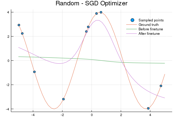
Here's the code used to generate the plot:

# These will be used in future model evaluations
x = rand(Uniform(-5, 5, 10)
testx = range(-5; stop=5, length=50)
wave = SineWave(4, 1)

# This model is not trained
random_model = Chain(Linear(1, 64, tanh), Linear(64, 64, tanh), Linear(64, 1))

data = eval_model(random_model, x, testx, wave, updates=32, opt=Descent(0.02))

p = plot_eval_data(data, "Random - SGD Optimizer")
plot(p)

Transfer Learning

This is essentially a standard training procedure:

function transfer_learn(model; opt=Descent(0.02), epochs=30_000,
                        train_batch_size=50, eval_batch_size=10, eval_interval=1000)

    weights = params(model)
    dist = Uniform(-5, 5)
    testx = range(-5, stop=5, length=50)

    for i in 1:epochs
        task = SineWave()
        x = rand(dist, train_batch_size)
        y = task(x)
        l = Flux.mse(model(x'), y')
        Flux.back!(l)
        Flux.Optimise._update_params!(opt, weights)

        if i % eval_interval == 0
            @printf("Iteration %d, evaluating model on random task...\n", i)
            eval_x = rand(dist, eval_batch_size)
            eval_model(model, eval_x, testx, SineWave())
        end
    end
end

The only difference from the random model code is transfer_learn is called after the model is initialized.

transfer_model = Chain(Linear(1, 64, tanh), Linear(64, 64, tanh), Linear(64, 1))
transfer_learn(transfer_model, epochs=50_000, opt=Descent(0.01))
...
p = plot_eval_data(data, "Transfer - SGD Optimizer")

Transfer learning doesn't fair any better than using a random model:

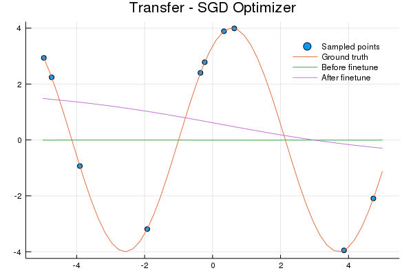
Transfer learned model finetuned on sine wave

Why? Let's examine the sine wave dataset. The model is learning to map a number to a number.

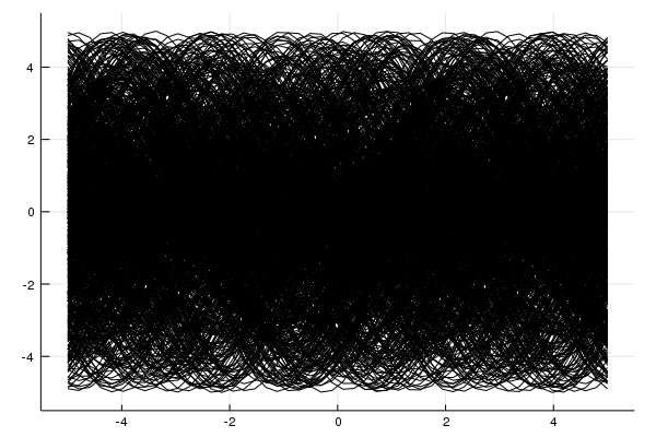
That's 1000 sine waves. See the problem? For every $x$ (input) value there's a line of possible $y$ (output) values, thus the model will simply learn to predict 0 - the expected value. Meta-learning models will learn to do the same, the difference being the representation learned is optimized to quickly learn a new task whereas the transfer learning representation does not.

MAML

By Mark Basarab on Unsplash

MAML can be succinctly described as:

\phi_i = \theta - \alpha \bigtriangledown_{\theta} Loss(D_{t_i}^{train}; \theta) \\ \theta \leftarrow \theta - \beta \sum_i \bigtriangledown_{\theta} Loss(D_{t_i}^{test}; \phi_i)

The first line shows the inner update, which optimizes $\theta$ towards a solution for the task training set $D_{t_i}^{train}$ producing $\phi_i$ . The following line is the meta update which aims to generalize to new data. This involves evaluating all $\phi_i$ on the test sets $D_{t_i}^{test}$ and accumulating the resulting gradients. $\alpha$ and $\beta$ are learning rates.

The difference between MAML and FOMAML (first-order MAML) is the inner gradient, shown is red is ignored during backpropagation:

\theta = \theta - \beta \sum_i \bigtriangledown_{\theta} Loss( \theta - \alpha {\color{red} \bigtriangledown_{\theta} Loss(\theta, D_{t_i}^{train})}, D_{t_i}^{test})

We'll focus on FOMAML since it's less computationally expensive and achieves similar performance to MAML in practice and has a simpler implementation.

FOMAML generalizes by further adjusting parameters based on how performance on a validation or test set (used interchangeably) during the meta update. This is best shown visually:

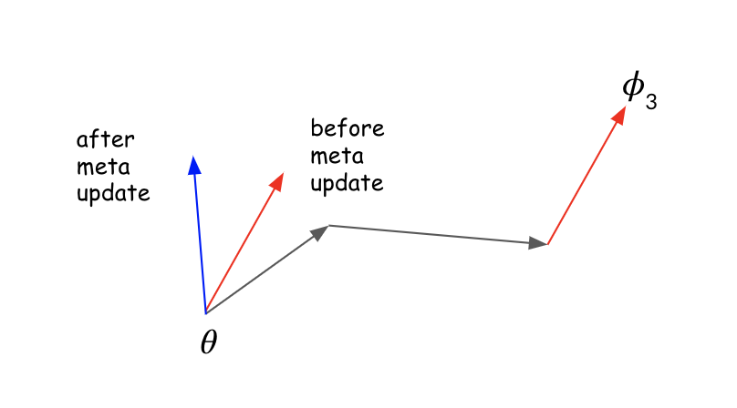
$\theta$ is the starting point, $\phi_{3}$ is the parameter values after 3 gradient updates on a task. Notice before the meta update the parameters shift in the direction of the new task's solution (red arrow) but after the meta update they change direction (blue arrow). This illustrates how the meta update adjusts the gradient for task generalization.

Here's the code:

function fomaml(model; meta_opt=Descent(0.01), inner_opt=Descent(0.02), epochs=30_000,
              n_tasks=3, train_batch_size=10, eval_batch_size=10, eval_interval=1000)

    weights = params(model)
    dist = Uniform(-5, 5)
    testx = Float32.(range(-5, stop=5, length=50))

    for i in 1:epochs
        prev_weights = deepcopy(Flux.data.(weights))

        for _ in 1:n_tasks
            task = SineWave()

            x = Float32.(rand(dist, train_batch_size))
            y = task(x)
            grad = Flux.Tracker.gradient(() -> Flux.mse(model(x'), y'), weights)

            for w in weights
                w.data .-= Flux.Optimise.apply!(inner_opt, w.data, grad[w].data)
            end

            testy = task(testx)
            grad = Flux.Tracker.gradient(() -> Flux.mse(model(testx'), testy'), weights)

            # reset weights and accumulate gradients
            for (w1, w2) in zip(weights, prev_weights)
                w1.data .= w2
                w1.grad .+= grad[w1].data
            end

        end

        Flux.Optimise._update_params!(meta_opt, weights)

        if i % eval_interval == 0
            @printf("Iteration %d, evaluating model on random task...\n", i)
            evalx = Float32.(rand(dist, eval_batch_size))
            eval_model(model, evalx, testx, SineWave())
        end

    end
end

Let's walk through this:

grad = Flux.Tracker.gradient(() -> Flux.mse(model(x'), y'), weights) is equivalent to torch.autograd.grad with create_graph=True. The gradients returned from Flux.Tracker.gradient are TrackedArray's which automatically keep track of operations for differentiation. In order to avoid this we can access the .data field which is a Array and does not track operations for differentiation.

for w in weights
	w.data .-= Flux.Optimise.apply!(inner_opt, w.data, grad[w].data)
end

Flux.Optimise.apply! computes the gradient given the optimizer which is then applied to the weights, w.data .-= ....

grad = Flux.Tracker.gradient(() -> Flux.mse(model(testx'), testy'), weights) is the gradient from evaluating $\phi_t$ on the test set.

Next we accumulate the gradients and reset the weights:

for (w1, w2) in zip(weights, prev_weights)
	w1.data .= w2
	w1.grad .+= grad[w1].data
end

Finally we update the original weights $\theta$ : Flux.Optimise._update_params!(meta_opt, weights).

Training with FOMAML:

fomaml_model = Chain(Linear(1, 64, tanh), Linear(64, 64, tanh), Linear(64, 1))
fomaml(fomaml_model, meta_opt=Descent(0.01), inner_opt=Descent(0.02), epochs=50_000, n_tasks=3)
...
p = plot_eval_data(data, "FOMAML - SGD Optimizer")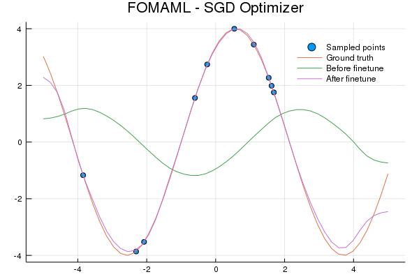

MAML learned model finetuned on sine wave

Reptile

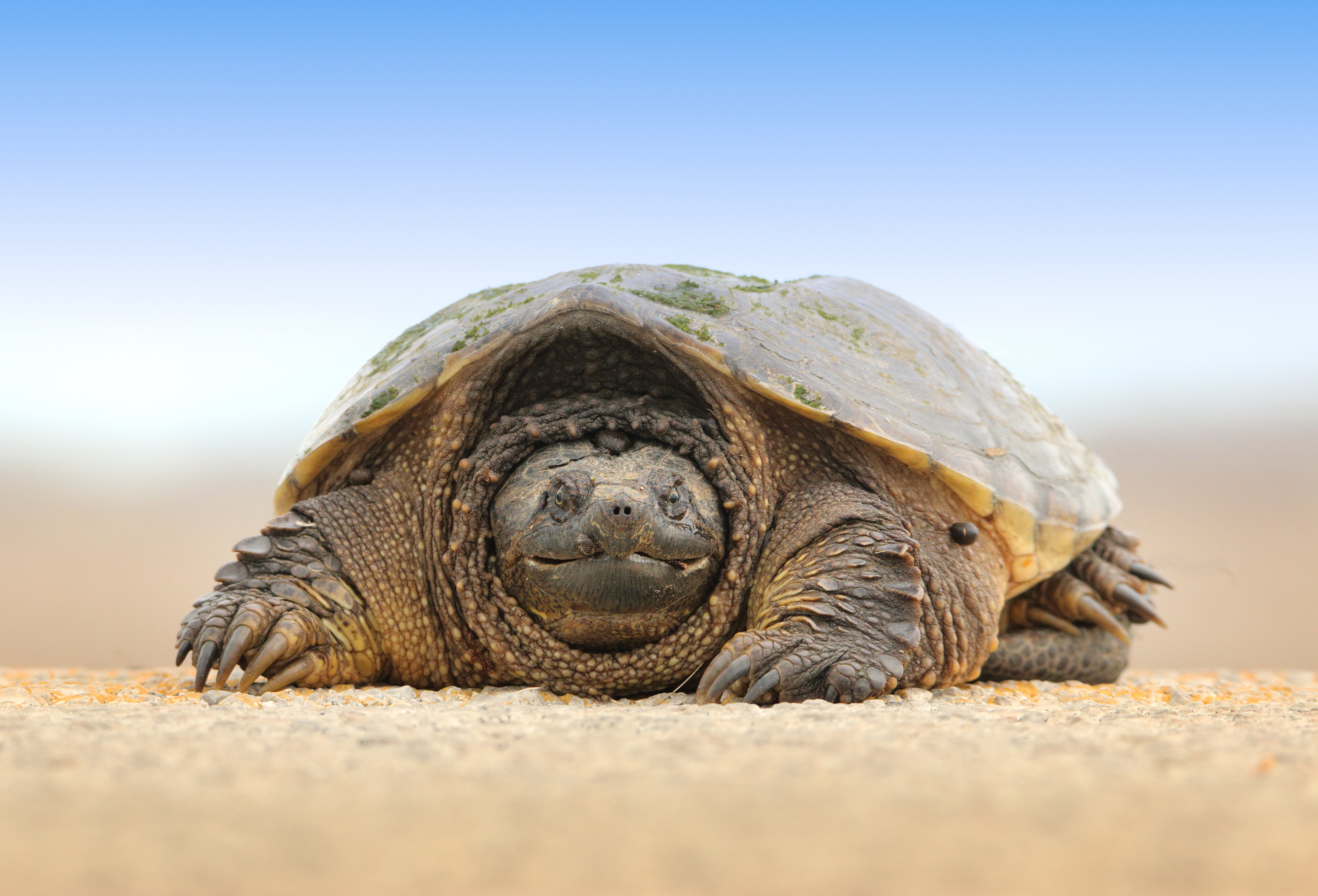
By Gary Bendig on Unsplash

Reptile optimizes to find a point (parameter representation) in manifold space which is closest in euclidean distance to a point in each task's manifold of optimal solutions. To achieve this we minimize the expected value for all tasks $t$ of $(\theta - \phi_{*}^{t})^2$ where $\theta$ is the model's parameters and $\phi_{*}^{t}$ are the optimal parameters for task $t$ .

E_{t}[\frac{1}{2}(\theta - \phi_{*}^{t})^2]

In each iteration of Reptile we sample a task and update $\theta$ using SGD:

\theta \leftarrow \theta - \alpha \bigtriangledown_{\theta} \frac{1}{2}(\theta - \phi_{*}^{t})^2 \\ \theta \leftarrow \theta - \alpha(\theta - \phi_{*}^{t})

In practice an approximation of $\phi_{*}^{t}$ is used since it's not feasible to compute. The approximation is $\phi$ after $i$ gradient steps $\phi_{i}^{t}$ .

The above figure shows the Reptile update. The red arrow is the direction of the gradient update. The blue arrow is the direction of the gradient update towards $\phi_{i}$ .

This a Reptile update after training for 3 gradient steps on task data. Note with Reptile there's no train and test data, just data. The direction of the gradient update (blue arrow) is directly in the direction towards $\phi_{i}$ . It's kind of crazy that this actually works. Section 5 of the Reptile paper has an analysis showing the gradients of MAML, FOMMAL and Reptile are similar within constants.

Here's the code for Reptile.

function reptile(model; meta_opt=Descent(0.1), inner_opt=Descent(0.02), epochs=30_000,
                 train_batch_size=10, eval_batch_size=10, eval_interval=1000)

    weights = params(model)
    dist = Uniform(-5, 5)
    testx = Float32.(range(-5, stop=5, length=50))
    x = testx

    for i in 1:epochs
        prev_weights = deepcopy(Flux.data.(weights))
        task = SineWave()

        # Train on task for k steps on the dataset
        y = task(x)
        for idx in partition(randperm(length(x)), train_batch_size)
            l = Flux.mse(model(x[idx]'), y[idx]')
            Flux.back!(l)
            Flux.Optimise._update_params!(inner_opt, weights)
        end

        # Reptile update
        for (w1, w2) in zip(weights, prev_weights)
            gw = Flux.Optimise.apply!(meta_opt, w2, w1.data - w2)
            @. w1.data = w2 + gw
        end

        if i % eval_interval == 0
            @printf("Iteration %d, evaluating model on random task...\n", i)
            evalx = Float32.(rand(dist, eval_batch_size))
            eval_model(model, evalx, testx, SineWave())
        end

    end
end

The only interesting bit here is the Reptile update:

for (w1, w2) in zip(weights, prev_weights)
	gw = Flux.Optimise.apply!(meta_opt, w2, w1.data - w2)
	@. w1.data = w2 + gw
end

The gradient is w1.data - w2 which pulls the parameters in the direction of the solution to the task $t_i$ .

Training using Reptile:

reptile_model = Chain(Linear(1, 64, tanh), Linear(64, 64, tanh), Linear(64, 1))
reptile(reptile_model, meta_opt=Descent(0.1), inner_opt=Descent(0.02), epochs=50_000)
...
p = plot_eval_data(data, "Reptile - SGD Optimizer")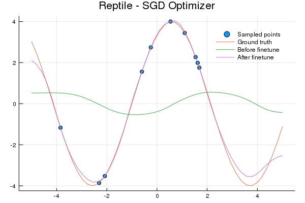

Reptile learned model finetuned on sine wave

Testing Robustness

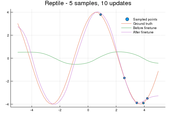
To test if the FOMAML and Reptile representations learned to learn quickly with minimal data we'll finetune on 5 datapoints for 10 update steps. The x values are sampled from a uniform distribution of [0, 5], the right half of the sine wave. Can the entire wave be learned?

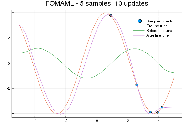
Lastly, let's see how quickly a representation is learned for a new task. We'll use the same 5 element sample as before and train for 10 gradient updates.

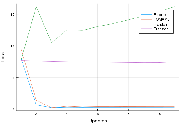
Cool! Both FOMAML and Reptile learn a very useful representation within a few updates. Both the transfer and random models perform poorly, as we would expect.

Notes

The sine wave problem is susceptible to loss divergence (loss -> inf). The Xavier initialization, especially for the initial layer, Linear(1, 64) seems to be particularly important. I tinkered with optimizers a fair amount, I was suprised ADAM didn't perform well.
Descent(0.02) performs much better than Descent(0.01) as the inner optimizer. I hypothesize this is due to the small amount of updates in the inner loop thus it's particularly important to learn quickly.
relu performs worse than tanh - the predicted sine wave isn't as smooth.
Learning the structure of a sine wave internally then scaling and shifting it during finetuning is super awesome.