All the code can be found here.
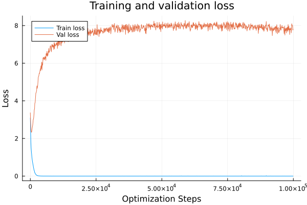
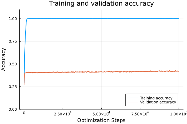
The "Grokking Paper" is one of the most head-scratching papers to come out in the neural network space. It explores the phenomenon of a regime change, whereby the model appears, by all indications, to have overfit the data, and that it's only being exacerbated as training progresses. Validation loss is increasing, and validation accuracy is at a standstill. Meanwhile, 100% training accuracy was hit ages ago. But then, all of a sudden, as if a divine entity itself sprinkled fairy dust on the neural network, validation loss begins to decrease and validation accuracy increases. After a while, both accuracies are at 100%. In essence, the neural network is transitioning from a regime of memorization to generalization.
Experiment Setup
The datasets are of the form:
where can be an arbitrary binary operation with a consistent modulus base. For the experiments this will be 97. For some operations this means the table has 97^2 = 9409 entries. Roughly. It could be 96^2 or 98^2. For others, negative numbers are also possible, so the space would be (assuming [-97, -96, ..., 96, 97]) 195 numbers and roughly 38205 table entries.
a, b, and c are placeholders but symbols are used to represent each number.
julia> alphabet = string.(vcat('a':'z', 'A':'Z', Char.(1024:2048)))

1077-element Vector{String}:
 "a"
 "b"
 "c"
 "d"
 ⋮
 "߽"
 "߾"
 "߿"
 "ࠀ"

julia>

julia> modn = 97
97

julia>

julia> nums = collect(-modn:modn)
195-element Vector{Int64}:
 -97
 -96
 -95
 -94
   ⋮
  94
  95
  96
  97

julia> num2tok = Dict{Int,String}()
Dict{Int64, String}()

julia> for (i, n) in enumerate(nums)
           num2tok[n] = alphabet[i]
       end

julia> num2tok
Dict{Int64, String} with 195 entries:
  56  => "ѥ"
  35  => "ѐ"
  60  => "ѩ"
  -5  => "Ш"
  67  => "Ѱ"
  73  => "Ѷ"
  -66 => "F"
  -71 => "A"
  ⋮   => ⋮

julia>

julia> tok2num = Dict(values(num2tok) .=> keys(num2tok))
Dict{String, Int64} with 195 entries:
  "Z" => -46
  "ф" => 23
  "Л" => -18
  "C" => -69
  "т" => 21
  "r" => -80
  "л" => 14
  "ѱ" => 68
  ⋮   => ⋮
And so the neural network will never see an actual number just the symbol that represents it.
The entire code for generating a dataset:
function create_dataset_binop_with_mod(f::Function, modn::Int)
    nums = collect(-modn:modn)
    num2tok = Dict{Int,String}()
    for (i, n) in enumerate(nums)
        num2tok[n] = alphabet[i]
    end

    tok2num = Dict(values(num2tok) .=> keys(num2tok))
    toks = collect(values(num2tok))
    push!(toks, "=")
    push!(toks, "∘")
    tok2idx = Dict(c => i for (i, c) in enumerate(toks))
    idx2tok = Dict(i => c for (i, c) in enumerate(toks))

    data = Vector{Int}[]
    for a in 1:modn
        for b in 1:modn
            c = f(a, b)
            # the operation is hidden from the model
            # all that's is the inputs and output
            s = "$(num2tok[a])∘$(num2tok[b])=$(num2tok[c])"
            # encode
            enc = [tok2idx[string(c)] for c in s]
            push!(data, enc)
        end
    end
    Random.shuffle!(data)

    X = zeros(Int, (length(data[1]) - 1, length(data)))
    y = zeros(Int, length(data))
    for (i, enc) in enumerate(data)
        X[:, i] = enc[1:end-1]
        y[i] = enc[end]
    end
    return (X, Flux.onehotbatch(y, 1:length(tok2idx))), tok2idx, idx2tok
end
This is the most important section:
c = f(a, b)
# the operation is hidden from the model
# all that's is the inputs and output
s = "$(num2tok[a])∘$(num2tok[b])=$(num2tok[c])"
The network only sees "SymbolA∘SymbolB=SymbolC".
The network itself is a two layer transformer with 128 dimensions split over 4 heads.
vocabsize = size(trainY, 1)
blocksize = size(trainX, 1)
# paper used 128 for embedding size and 4 heads
dembed = 128
nheads = 4
nlayers = 2
circ = Circuit(vocabsize, blocksize, dembed; nheads, nlayers) |> gpu;
opt = Flux.setup(AdamW(3e-4), circ);
The vocabulary size is the 195 symbols plus 2 extra for and .
The block size is 4 (all tokens before SymbolC).
Data Split
Memorization -> generalization is established due to the dataset split. For the experiments we'll do it's a 50/50 split. Meaning half of the data the neural network will have never seen. It cannot, by definition memorize it. The only way for it to correctly label the examples in the validation set is to figure out the underlying function being performed. To generalize.
X, Y = data;
trainfrac = 0.5;
N = size(X, 2);
n = Int(round(N * trainfrac));
trainX, trainY = X[:, 1:n], Y[:, 1:n];
valX, valY = X[:, n+1:N], Y[:, n+1:N];

trainX = trainX |> gpu;
trainY = trainY |> gpu;
valX = valX |> gpu;
valY = valY |> gpu;

train_batchsize = min(512, size(trainX, 2))
val_batchsize = min(512, size(valX, 2))
traindata = Flux.DataLoader((trainX, trainY), batchsize = train_batchsize, shuffle = true);
valdata = Flux.DataLoader((valX, valY), batchsize = val_batchsize);
In the original paper they run experiments over a variety of functions and split sizes. I've picked four functions from the paper I thought would be worthwhile reproducing.
Each of these had a 50/50 split except the last one which I also tried with a 95/5 split, as they did in the paper. It failed to generalize in the paper and it failed to generalize for me :(
The results ...
Run It
data, _, _ = create_dataset_binop_with_mod((a, b) -> (a + b) % modn, modn)

...

run = Run()
evalevery = 10
train_model!(
    circ,
    opt,
    traindata;
    nepochs = 10_000,
    evaliters = 10,
    evalevery = evalevery,
    valdata = valdata,
    seq2val = true,
    early_stop = () -> begin
        # stop if the validation accuracy is >= 0.99
        accuracy_metric(circ, valdata; seq2val = true) >= 0.99
    end,
    run = run,
)
Nothing out of the ordinary here. evaliters defines the interval which the loss and accuracies for the train and validation data should be captured. Every 10 epochs.
seq2val means we only care about the loss for the last token, rather than seq2seq, which would be the loss for token prediction in the entire sequence.
    f = if seq2val
        (m, x, y) -> Flux.Losses.crossentropy(softmax(m(x), dims = 1)[:, end, :], y)
    else
        (m, x, y) -> Flux.Losses.crossentropy(softmax(m(x), dims = 1), y)
    end
In Julia arrays are column ordered so the batch and sequence dimensions would be the final two -
(..., ..., sequence_dim, batch_dim). This is the opposite of PyTorch.
If you read my notes in the grokking.jl you'll see I originally had seq2seq loss, mainly because I was working with seq2seq data before but also because of I was too lazy to change the loss metric. It does hurt the model in this case because it's not useful for it predict any of the tokens besides the final one.
Given the first three tokens you will not be able to predict the fourth token. It could be any of the number symbols (excludes and ) will equal probability!
Anyway - back to modular addition.
Plots, plots, plots.
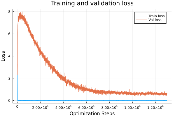
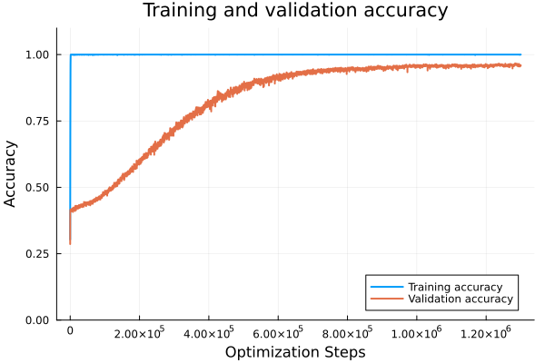
Addition
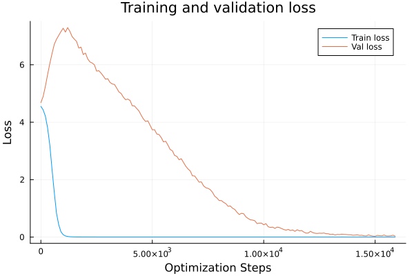
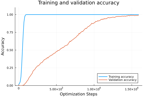
Total Optimization steps are defined as epochs _ num_batches _ evalevery. So addition generalizes pretty quick but the regime change from memorization to generalization is evident.
Subtraction
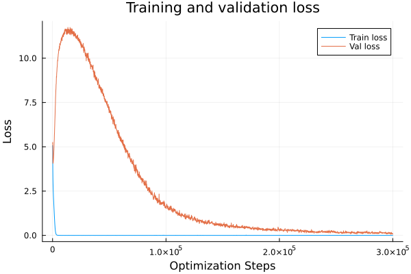
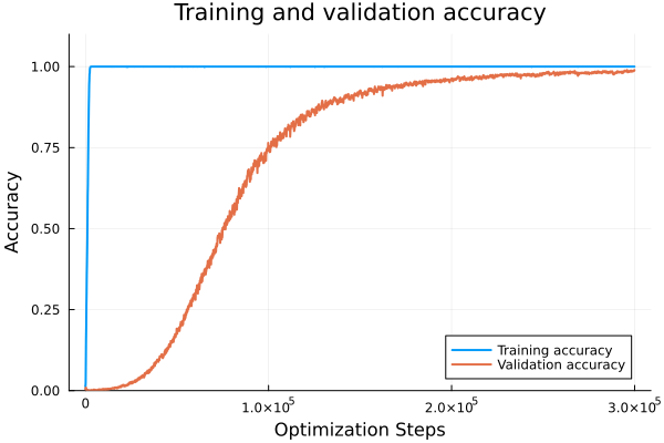
Generalization takes much longer than addition.
Asymmetric Function
I stopped this early at around 95% validation accuracy just because it was taking so longbut. Validation loss and accuracy were going down the entire duration after the regime change.
Hard Function
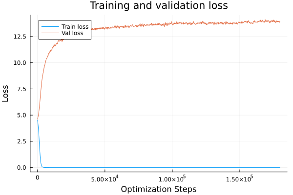
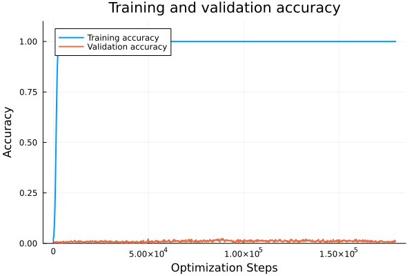
Even with a 95/5 split we get nowhere.
Extra: Subtraction then Finedtuned Asymmetric
I took the subtraction model once it achieved high generalization and then attempted to finetune it on the asymmetric dataset. It did not work.
Value Counts
I'm not sure how useful this is these visualizations show a correlation between symmetry and the ability to generalize.
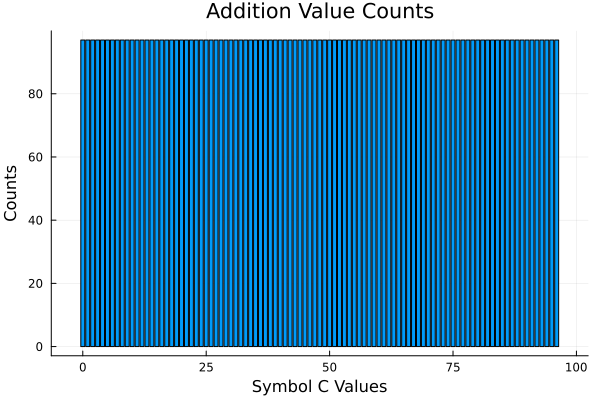
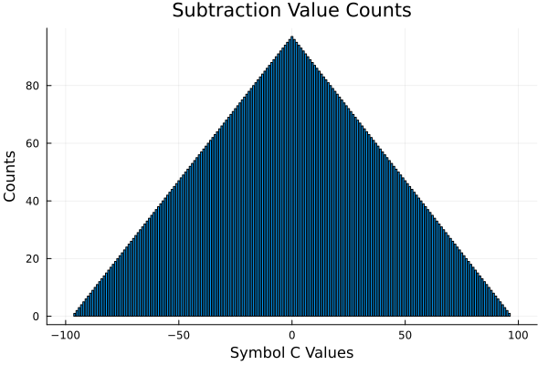
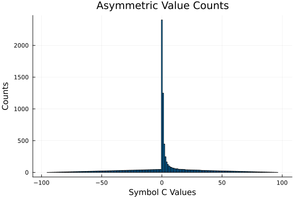
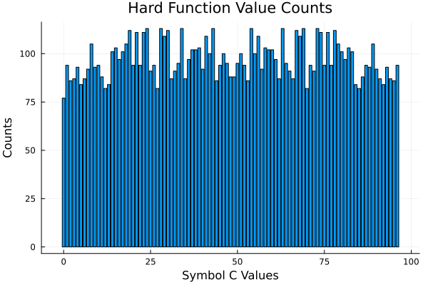
Even the hard function does have symmetry. Hmmmmm.
Next Steps
These neural networks are fairly small so dissecting them could be worthwhile.